While the ability to create your own formulas in Excel is powerful, it is time consuming (not to mention that it requires that you know the formula!). The people at Excel realize this and have created a set of formulas (they call them functions) ready for you to use. There are several hundred predetermined functions in Excel, one of them is the SUM function (which sums a series of cells).
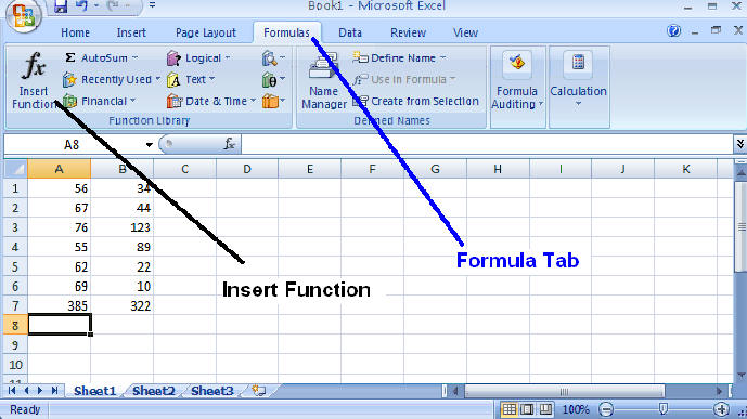
In your spreadsheet, select the cell A8. To access the formulas, select the FORMULA tab at the top of the page and select INSERT FUNCTION as shown in the following figure.
You should now get the FUNCTION dialog box which is shown below.
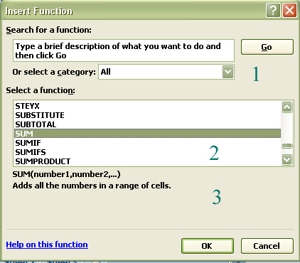
In the category select window (labeled 1 in the figure), select All (as shown). As you become familiar with the different categories, you can use them to make your search a bit easier, but for now, we know that all the functions will be found in the All category. Scroll down the selection window (section 2) until you reach the SUM function and highlight it with a single mouse click (as shown in the figure). The functions are sorted in alphabetical order, so you will need to scroll down to the S's. Note that a brief description of the function is shown in section 3 of the dialog box. With the SUM function selected, press the OK button. You will now see a new dialog box titled FUNCTION ARGUMENTS. In this dialog box, you will indicate which numbers you want summed. This box is shown below:
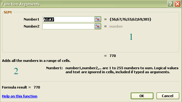
The important section is the input box (number 1 in the figure). As you should see, Excel automatically inputs a range of values that it thinks you want summed. In this case, it is the column of number above the cell containing the function (A8 in this case) - A1:A7. The colon (:) is the Excel convention to indicate all cells between A1 and A7 inclusive. One could also write this by typing all cells individually, but the shortcut is easier. Note, this is not the range of cells you want to sum as it includes A7 (which is the sum function you previously created) - you do not want to include this in the sum. In other words, you want the sum of A1:A6. Use the mouse and click on the first input box (labeled Number 1) so that the cursor is blinking to the right of the 7. Use the backspace to erase the 7 and replace it with a 6. The input box should now read A1:A6, which is the range you want to sum. By the way, suppose you wanted to sum all the numbers in rows 1-6 of both columns (A and B). You can input the B column range in the window 'Number 2' by clicking on the window and typing B1:B6. You will notice two thing after doing this, one is that the sum (shown next to 2 in the dialog box) is now 707 and that a third input window is formed. You can add up to 30 (I think) different input windows. Delete the values in "Number 2" but make sure that the cursor in blinking in that window. Here is another way to input values into an input window. With the cursor blinking in the "Number 2" window, use your mouse and highlight the cells B1-B6 (highlight by clicking on B1 and drag the cursor down to B6 - do not release the mouse button until you reach B6 - and do not 'drag the box', you do not want to change the values in the cells). When you finish, you will find that the highlighted cells are now included in the input box. I find that this is generally the easiest way to input values into input windows. Now, delete all values in 'Number 2" and press the OK button. You should find the value in A8 is equal to that in A7. "Drag the box" and copy A8 into B8. Your screen should look like this:
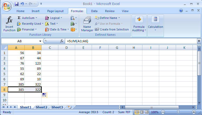
Note the function listed in the formula bar.
Now, insert 6 values of your own choosing and place in the first 6 rows of column D. Sum the column in D7 (the hard way) and D8 (the function way). In cell E2, please sum all the values in cells A1-A6, B1-B6 and D1-D6 for a grand total.