To insert data, you simply use your mouse to select a cell and then simply type. Start the Excel program. Select the cell A1 (that is the cell in column A, row 1) by using your mouse and clicking the left mouse button (this is the 'normal" mouse button). Note that the name of the cell is displayed in the Name Box. By default, the name of the cell is its address with reference to the row/column although you can name a cell anything you want using the Insert/Name menu item..
56, 67, 76, 55, 62, 69.
To do this, simply select the cell (A1 should already be selected) and type in the number 56 and press the ENTER key. This will insert the number 56 into cell A1 and automatically move the active cell to A2. Now type in 67 into A2, and press enter. Continue in this fashion until all six numbers are inserted in the first 6 rows of column A.
34, 44, 123, 89, 22, 10
WARNING NOTE: In many instances, you will be using numbers with units (like meters, or grams). When using Excel, never mix numbers with letters in a cell. If you do, Excel assumes that you are inserting text and not inserting numbers. For example, if the units for the numbers you inserted in the previous example are grams, do not type 34 g (or 34 grams) in a single cell - Excel will not recognize this as a number. This is probably the primary reason for student errors when analyzing data in Excel. Now, simply type 34. You can use a label on the column to indicate the units. You will learn later how to insert a label.
That should have been easy - now lets do some calculations.
Let's add the numbers in each column and place the sum in the 7th row of each column. One way (the hard way) would be as follows:
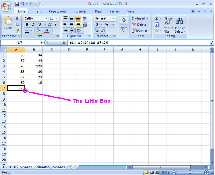
Note that the sum of the numbers in column 1 is displayed in cell A7 and that the formula is shown in the window of the formula bar. If you were to change the value of cell A1 from 56 to 55, you would find that the sum shown in A7 would also change. (Try it, but remember to change it back). NOTE: If you were to forget to start the formula with the equal sign, Excel would assume that you are typing in text and would not do any calculations!
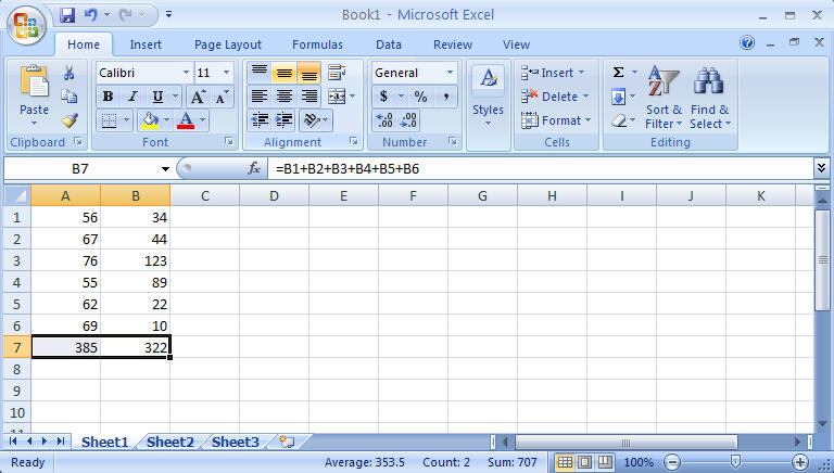
One can do the same procedure to sum the values in column B and type =B1+B2+B3+B4+B5+B6 into cell B7 (actually, you could type it into any cell, but it is more logical to use B7). But there is an easier way. Note that there is small box in the lower right corner of any selected cell. Select cell A7 (as shown above) and move, without pressing a button, the cursor over the box. You should note that the cursor changes when over the box, changing from a hollow cross to a simple line cross. This will occur automatically whenever the cursor lies over the little box. Do this several times so that you are familiar with its appearance.
Now, with the cursor over the box in cell A7 (and thus in the line format), press down and hold the left mouse button and drag the mouse over cell B7. Once you observe that B7 becomes selected, release the button. If done correctly, you should find that the formula was copied into B7 but that it changed so that it summed the contents of Column B! Pretty amazing! Your screen should look like the following figure (with cell B7 selected). This is much easier than typing in all of the cell names into the formula. This process (where you use the little box to copy a formula to adjacent boxes) will be know as "dragging the box" in this tutorial.