
Scientists used statistics to summarize their data (making it easier to present their data) and to help them make conclusions based on their data. A description of these statistics is described in your lab manual.
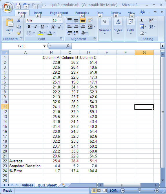
In this quiz, you must download this Excel file. When you open the file, you will find that there are two sheets, one named "values" the other is named "Quiz Sheet" - see the tabs at the bottom. There are three columns of data on the "values" while the other sheet is empty - the values sheet is shown below. Your values will not be the same as the ones shown here.
Highlight all the data, including the column labels and use the "copy" function to copy the data to the clipboard. Go to "Quiz Sheet" and highlight A1. On the left hand side of the HOME tab are the copy and paste buttons. Use the the copy command to copy the data. To paste, click on the small arrow just below the word PASTE and choose paste special. You will then get a dialog box - select values - this will then paste all the data into the first three columns of the new sheet. Before doing anything else, make sure you copy the data to the "Quiz Sheet". If you do not do this exactly as describe above, the numbers that you pasted will change on you and you will go crazy. Also, the numbers on the values sheet will continue to change - there is nothing you can do about it. This will not affect your work as once you properly copy values to the Quiz Sheet, you never need to use the values sheet again.
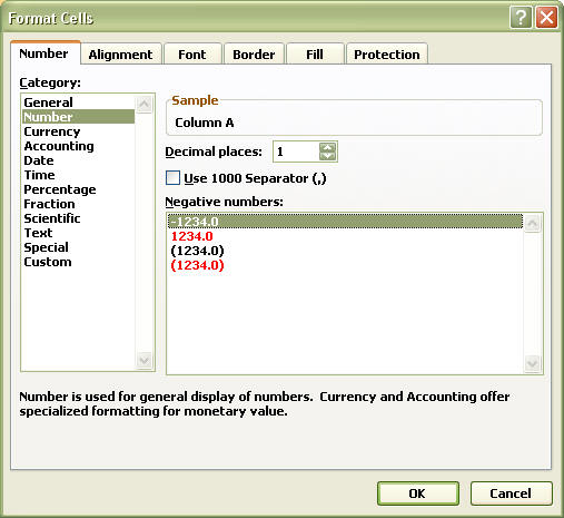
Format each cell so that each cell has only 1 decimal point. One way to do this is to highlight on all the cells that you wish to format, right mouse click on the highlighted cells, and you will see the menu shown in the figure below. Select Format Cells.

You will then get the following dialog box. In the Category box, select number and set Decimal Places to 1 (as shown in the figure). Press OK and you will now find that numbers have just 1 decimal place!
There are 20 values for each column, extending from row 2 to row 21. You are to use the built in functions of Excel to calculate the average (avg) and the standard deviation (stdev). Place the average of each column in row 22 (so that they lie directly below the set of data) and the standard deviation in row 23. You must format the table (in any clear way) so that you can label row 22 so that the reader will know that it is the average (and so the same with standard deviation). Please format the all formula cells so that there is only 1 decimal place and so the font is NOT black (all other values should be left black). You may use any color as long as the numbers are readable and the same color is used for all formula cells. This is done using the format cells menu that you used to set the number of decimal places. Select the font tab to change the font attributes (including color). One example is shown below.
There is no built-in function for percent error, so you must create the formula. Let us assume that the actual values for each column should be 25. You can now use the average that you calculated for each column to calculate the percent error. Remember that percent error or the mean is equal to the absolute value of ((calculated mean - actual value)/actual value) * 100. Select cell A 24 and type in the label "Percent Error". Enter the formula for the percent error in cell B 24. Remember that all formulas must start with an equal sign - so type =((B22-25)/25)*100 and press the ENTER key - this will then calculate the percent error for the average of the values in column B. Drag the box to copy the formula to column C and D.
Next, you must perform the t-test to determine if the various columns are significantly different.